In earlier versions of TPoint, a pointing model beyond the six standard geometrical terms had to be constructed “manually” based on the rules outlined in section “Adding Terms” on page 548.
While the models developed using this technique often achieved accurate pointing results, the process proved to be somewhat daunting and error prone for many, especially beginners.
One looming question always seemed to remain, “How do I really know that I’m getting the best pointing for my imaging system?”
TPoint’s Super Model feature answers the question above by determining the optimal pointing model for you. Clicking the Super Model button (page 489) performs an extensive statistical analysis of the pointing calibration data and converges on the optimal pointing model using all the processing power of your computer.
The Super Model algorithm goes far beyond the iterative approach discussed above and removes the drudgery of creating a pointing model.
Patrick Wallace, the TPoint and Super Model author, comments:
“The modeling has to explore a large multidimensional parameter space, applying strict statistical tests, and despite a myriad of optimizations this inevitably means a large amount of processing time. The application is extremely careful about efficient use of machine resources; the length of time the computations take is purely a reflection of the difficulty of the task.”
The length of time required to find the Super Model mainly depends on:
· The number of calibration points in the pointing calibration run. (For best results, use at least 40 calibration points, distributed on both sides of the meridian.)
· The speed of the computer’s CPU.
· For computers that have multiple CPU, the more CPUs, the less time required (provided the Use All CPUs checkbox is turned on, see page 489).
· The operating system and the operating system’s architecture (32- or 64-bit).
Computing a Super Model for 250 calibration points on a Windows 7 64-bit 4 CPU machine the takes about 55 seconds. Large calibration runs (up to 1000 points maximum) on a single CPU can take more than 10 minutes. An 830-calibration point run on an eight-CPU 2.93 GHz Windows 7 64-bit machine using all 8 CPUs takes just over 120 seconds.
The resulting Super Model will shed light on the integrity of your imaging system. If the TPoint model shows an RMS of about 15 arcseconds or better for a permanently mounted system, you’ve most likely reached the “best pointing possible for an amateur telescope” limit. If the RMS pointing is greater than about 30 arcseconds or so for a permanently mounted system, or greater than one arcminute for a portable system, and you want to do better, it’s time to analyze every single component of your imaging system do determine the source of the pointing errors.
· Is the telescope’s mirror fixed? Mirror slop will introduce pointing errors. If possible, fix the mirror in place to minimize this error.
· How is the optical tube assembly attached to the mount? OTA mounting rings provide the most repeatable and reliable pointing. Dovetail mounting introduce flexure and can degrade pointing accuracy.
· How is the mount attached to the pier? Make sure all mounting bolts are tight so that the mount cannot move when the equipment is slewed to different parts of the celestial sphere.
· How is the pier attached to the ground? A solid and rigid mounting to a concrete foundation is critical.
· Are cameras, guiders, focusers, filter wheels and other devices mounted to the OTA bending, flexing or shifting as the mount slews to different areas of the sky?
· How much backlash is in the mount’s gears?
The ultimate question you must answer is, “How accurate does my pointing need to be for my imaging system and my observing goals?” No matter what the answer, the TPoint module will help you achieve your goals.
The following example shows the pointing accuracy obtained with a high-quality imaging system. The pointing calibration data was collected using the Automated Calibration feature (see “Automated Pointing Calibration” on page 508) on a permanently mounted, accurately polar aligned Paramount ME carrying a ring mounted C-14 with the mirror locked in place. The SBIG ST-8 was rigidly attached to an Optec TCS focuser and all cables routed so that there was no drag or sag on the system.
Note that the 831 pointing samples are used for demonstration purposes only. A 300-calibration point run produces similar pointing accuracy, as well as excellent ProTrack results on Paramount mounts. A point of diminishing returns is reached above about 300 pointing samples.
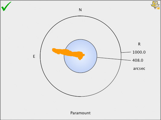
Figure 228: A scatter plot of 831 calibration points, with no terms in the model.
Figure 228 shows a scatter plot of the system’s pointing accuracy with no terms in the pointing model. With no TPoint modeling, pointing accuracy is 408 arcseconds (6.8 arcminutes) RMS. Not great pointing, for sure.
Remember, this data was acquired using a high-quality imaging system with minimal hysteresis, but the pointing accuracy is degraded by inherent “errors” from the optical and mechanical axis misalignments, gear errors, and so on. In other words, even with a “high-end” imaging system, the blind pointing accuracy will not be sufficient to routinely place objects in a relatively small field of view.
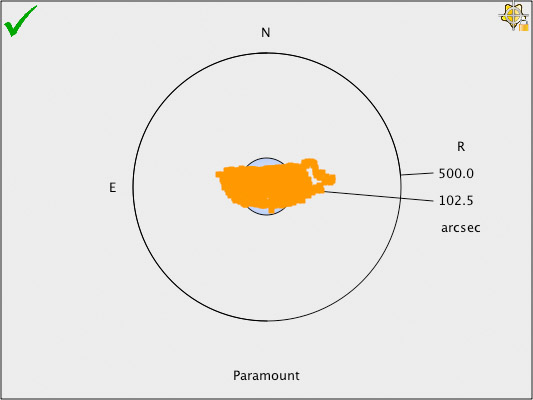
Figure 229: The pointing accuracy improves significantly using the six geometric terms.
Figure 229 shows that the pointing accuracy is improved significantly by adding the six standard geometric terms (IH, ID, NP, CH, ME and MA). The model’s RMS pointing is now 102.5 arcseconds (1.7 arcminutes). Better, not quite super.
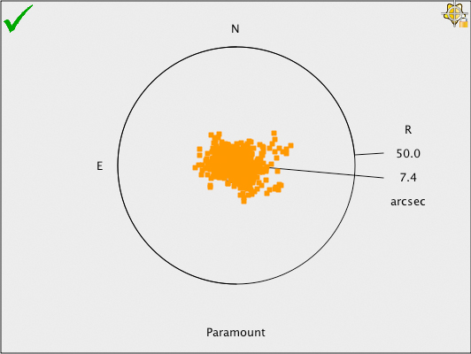
Figure 230: Scatter diagram showing pointing after applying a Super Model.
Figure 230 shows the scatter plot after applying the terms from the Super Model. The RMS pointing is now just over 7 arcseconds. This means that every object will be placed near the center of a 6 x 10 arcminute field of view.
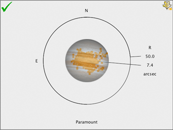
Figure 231: Scatter diagram with the planet Jupiter superimposed for scale. (Jupiter’s apparent size varies from about 30 arcseconds to about 50 arcseconds.)
Figure 231 shows the approximate relative size of the planet Jupiter on the scatter plot. Now that is super pointing accuracy!
After you have collected approximately 40 calibration points, click the Super Model button on the Model tab of the TPoint Module window to create the optimal pointing model.
After the Super Model has been computed, click the Apply button on the Super Model window so that TheSky will use this model to improve the telescope’s pointing.
|
|
Make sure that the Apply Pointing Corrections checkbox on the Setup pane of the TPoint Module window is turned on, otherwise, pointing corrections will not be applied when the telescope is slewed from TheSky. |


Figure 232: The Super Model button, highlighted in red, is located on TPoint Module > Model tab.
Turn on this check box to use all the available central processing units (CPUs) on your computer when computing the Super Model. Please see “Super Model and Parallel Processing” on page 492 for an in-depth discussion on this subject.
The Super Model Status window shows the progress and the total run time in minutes and seconds. Depending on the speed of your computer, computing a super model can take several minutes or more.
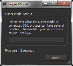
Figure 233: The Super Model Status window.
Click the Abort button on the Super Model Status window to end the computation process.
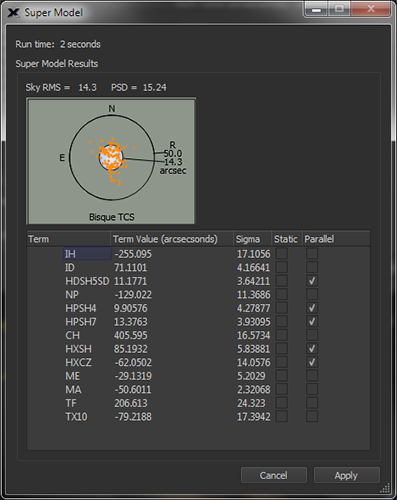
The Super Model Window shows the total run time, and the Super Model results.
|
Figure 234: The Super Model window showing the optimal model for the calibration data set. |
Click the Apply button to update the terms in the TPoint model to use the Super Model.
Computing a Super Model is an extremely processor intensive process, and the more pointing samples, the more time required to determine the solution. If your computer has multiple processors, turn on the Use All CPUs checkbox (page 489) to divide the work across every processor.
|
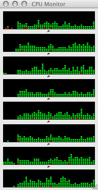
Figure 235: The Mac CPU Monitor Window showing the CPU usage during a Super Model run (eight CPU machine). |
Figure 235 shows the Mac’s CPU monitor window during a Super Model run. The graphs of the CPU usage show that, while every processor is being used, not 100 percent of the processing capability each CPU is utilized. The obvious question is, “Why not?” The following analogy attempts to explain why optimal parallel processing isn’t always possible for a given task.
Take, for example, the process of shutting down an observatory that has a roll off roof, where the entire process consists of two tasks (shown in the table below):
|
Task |
Description |
Time to Complete (seconds)* |
|
|
1 |
Slew the mount to the park position |
30 |
|
|
2 |
Close the roll off roof |
30 |
|
|
*For this example, we assume that each task cannot be completed in less time.
|
|||
|
Case A |
If both tasks can be run simultaneously, the time to shut down the observatory is 30 seconds
|
||
|
Case B |
If the roll off roof can strike mount unless the mount is at its park position, both tasks cannot be run simultaneously. Task 2 must follow the completion of Task 1. So, the time required to shut down the observatory in this case is 60 seconds. |
||
Most sophisticated computations like Super Model are analogous to case B. In other words, parallel processing is prohibited because of the nature of the algorithm where tasks and or computations depend on an earlier computation being completed first. Only when computations are completely independent can they be run in parallel.
|
Question |
Answer |
|
What is the minimum number of calibration points required by Super Model? |
While a Super Model can be applied to any number of calibration points, for best results, acquire a minimum of 40 calibration points that are distributed on both sides of the meridian.
Fewer than 40 points is not enough to let Super Model “get into its stride,” as it must settle for a very cautious model using only a handful of terms. At 40 points and higher, Super Model will use more terms and best cope with the whole sky.
|
|
There are terms used in the Super Model that don’t seem to apply to my imaging system. Should I remove them? |
For optimal pointing accuracy, the best practice is to use all the terms in the Super Model and not make any adjustments. To achieve optimal pointing, the Super Model algorithm: · Removes statistically invalid points · Adds terms to the model in the specific (optimal) order · Fixes specific terms in the model · Adds terms in parallel
Changing, adding, or removing terms makes the Super Model less effective.
|
|
My computer has eight CPUs, why isn’t Super Model eight times faster when the Use All CPUs checkbox is turned on?
|
Given the nature of the Super Model algorithm, fewer than 50% of the computations can be performed in parallel (see the observatory shut down analogy above). Therefore, on a given computer, the best possible speed increase is about 50%, or nearly two times as fast.
|
|
When computing a Super Model, not every computer core is used. Is this normal? |
Given the nature of the Super Model algorithm, fewer than 50% of the computations can be performed in parallel (see the observatory shut down analogy above). Moreover, for this particular task, the parallel computations are short lived, and the overall algorithm goes in and out of serial and parallel processing as necessary. Pegged CPUs do not tell the whole story; the Super Model Total Run Time when the Use All CPUs checkbox is turned on and off reveals the benefits of parallel processing for this task.
|
|
How do you compute how many times faster the Super Model is using all CPUs? |
For a given set pointing calibration data, run the Super Model with the Use All CPUs checkbox turned on and off and compare the Run Times (see Figure 234).
Run Time using a single CPU = 100 Run Time using all CPUs = 50 Times Faster = (100-50)/50 = 2
The inverse of this result is the percent faster: ½ = 50% faster. |
